site_name = "Heron 1"
sid = 1
ph = 8.1
alert = False

print("Site:", site_name)
print(f"ID: {sid}")
print(f"pH:{ph:.2f}")
print(alert)

type(sid)
type(alert)
Site: Heron 1
ID: 1
pH:8.10
FalseboolInstructor: Dr Nate Butterworth (Google XWF)
Date: May 7, 2026
Recoding: https://youtu.be/ENOLU_7OkE0
Note: we won’t explicitly cover best-practice coding style and conventions, read more in the Python Style Guide.
Visit Google Colab and start a “New notebook in Drive”.
There are many places the Python programming language exists and many ways to use it. We will be uing something called a “Python (Jupyter) Notebook” hosted on Google Colab. This has everything you will need pre-installed and immediately lets you run code and visualise your progress without too much setup.
Shift + Enter to run the current cell and move to the next.File > Save a copy in Drive.What are variables?
Think of variables as labels for containers that store data. You assign a value to a variable using the equals sign =.
Naming conventions:
sample_id instead of s)._).sample_id is different from Sample_ID).list, id, type).Common Data Types:
int): Whole numbers, e.g., 42, -10.float): Numbers with a decimal point, e.g., 3.14, -0.001, 2.0.str): Text, enclosed in single quotes ('...') or double quotes ("..."), e.g., "DNA", 'Escherichia coli'. Use f-strings for powerful string output formatting optionsbool): Represents truth values, either True or False.We can use the type() function to check the data type of a variable.
site_name = "Heron 1"
sid = 1
ph = 8.1
alert = False
print("Site:", site_name)
print(f"ID: {sid}")
print(f"pH:{ph:.2f}")
print(alert)
type(sid)
type(alert)Site: Heron 1
ID: 1
pH:8.10
Falsebool# Create variables for a gene sequence
gene_id = "BRCA1"
chromosome = "17" # Chromosomes can be numbers or letters (e.g., "X", "Y"), so they are stored as strings
genome_size_bp = 3100000000 # Human genome size in base pairs (large integer)
gc_content = 41.5
is_pathogenic = True
# Print the variables using different formatting options
print("Gene ID:", gene_id)
print(f"Chromosome Location: Chr {chromosome}")
print(f"Human Genome Size: {genome_size_bp:,} base pairs") # f-string with thousands separator
print(f"GC Content: {gc_content}%")
print(f"Is pathogenic? {is_pathogenic}")
# Print the data types
print("\nData types of variables:")
print(f" gene_id: {type(gene_id)}")
print(f" chromosome: {type(chromosome)}")
print(f" genome_size_bp: {type(genome_size_bp)}")
print(f" gc_content: {type(gc_content)}")
print(f" is_pathogenic: {type(is_pathogenic)}")Gene ID: BRCA1
Chromosome Location: Chr 17
Human Genome Size: 3,100,000,000 base pairs
GC Content: 41.5%
Is pathogenic? True
Data types of variables:
gene_id: <class 'str'>
chromosome: <class 'str'>
genome_size_bp: <class 'int'>
gc_content: <class 'float'>
is_pathogenic: <class 'bool'># Create variables for a patient health record
patient_id = 42 # An integer patient ID we want to format with zero-padding
patient_name = "Alex Doe"
temperature_c = 37.25 # High-precision Celsius reading
heart_rate_bpm = 75
is_stable = True
# Print the variables using advanced f-string formatting
print(f"Patient ID: PAT-{patient_id:04d}") # Formatted with zero-padding (PAT-0042)
print("Patient Name:", patient_name)
print(f"Temperature: {temperature_c:.2f} °C") # Formatted to 2 decimal places
print(f"Heart Rate: {heart_rate_bpm} BPM")
print("Is stable?", is_stable)
# Print the data types
print("\nData types of variables:")
print(f" patient_id: {type(patient_id)}")
print(f" patient_name: {type(patient_name)}")
print(f" temperature_c: {type(temperature_c)}")
print(f" heart_rate_bpm: {type(heart_rate_bpm)}")
print(f" is_stable: {type(is_stable)}")Patient ID: PAT-0042
Patient Name: Alex Doe
Temperature: 37.25 °C
Heart Rate: 75 BPM
Is stable? True
Data types of variables:
patient_id: <class 'int'>
patient_name: <class 'str'>
temperature_c: <class 'float'>
heart_rate_bpm: <class 'int'>
is_stable: <class 'bool'>Python supports various operators for performing calculations and comparisons.
Arithmetic Operators:
+ (addition)- (subtraction)* (multiplication)/ (division - always results in a float)// (floor division - discards the fractional part)% (modulo - remainder of a division)** (exponentiation - raise to the power of)Comparison Operators: (Result in a Boolean: True or False)
== (equal to)!= (not equal to)> (greater than)< (less than)>= (greater than or equal to)<= (less than or equal to)Logical Operators: (Combine Boolean values)
and (True if both are True)or (True if at least one is True)not (Inverts the Boolean value)# Calculate temperature anomaly above a threshold
start_temp = 28.0 # Degrees Celsius (but Python does not intrinsically know what units)
new_temp = 29.5
anomaly = new_temp - start_temp
print(f"T Anomaly: {anomaly:.1f} (C)")
# Check if it's above the bleaching threshold (e.g., 1.0 C)
bleach_thresh = 1.0
is_at_risk = anomaly >= bleach_thresh
print(f"Is reef at risk? {is_at_risk}")T Anomaly: 1.5 (C)
Is reef at risk? True# Exercise 1.2: Basic Operations (Genomics)
# Calculate GC content count and percentage
sequence_length = 5589
gc_count = 2320
# Calculate percentage of GC and AT bases
gc_percent = (gc_count / sequence_length) * 100
at_percent = 100.0 - gc_percent
# Check if sequence has high GC content (>50%) AND is a long sequence (>5000 bp)
is_high_gc = gc_percent > 50.0
is_long_sequence = sequence_length > 5000
is_target = is_high_gc and is_long_sequence
print(f"In a DNA sequence of length {sequence_length} bp:")
print(f"GC Count: {gc_count} bases ({gc_percent:.2f}%)")
print(f"AT Count: {sequence_length - gc_count} bases ({at_percent:.2f}%)")
print(f"Is high GC (>50%)? {is_high_gc}")
print(f"Is long sequence (>5000 bp)? {is_long_sequence}")
print(f"Meets target criteria (High GC AND Long)? {is_target}")In a DNA sequence of length 5589 bp:
GC Count: 2320 bases (41.51%)
AT Count: 3269 bases (58.49%)
Is high GC (>50%)? False
Is long sequence (>5000 bp)? True
Meets target criteria (High GC AND Long)? False# Exercise 1.2: Basic Operations (Health)
# 1. Calculate Mean Arterial Pressure (MAP)
# Formula: MAP = (Systolic BP + 2 * Diastolic BP) / 3
systolic_bp = 122
diastolic_bp = 82
map_value = (systolic_bp + (2 * diastolic_bp)) / 3
# Check if patient has elevated Mean Arterial Pressure (>= 100 mmHg)
is_map_elevated = map_value >= 100.0
print(f"Blood Pressure Reading: {systolic_bp}/{diastolic_bp} mmHg")
print(f"Calculated Mean Arterial Pressure: {map_value:.1f} mmHg")
print(f"Is patient's MAP elevated? {is_map_elevated}")
# 2. Calculate maximum heart rate and target exercise heart rate (75% intensity)
# Formula: Max HR = 220 - age
patient_age = 45
max_hr = 220 - patient_age
intensity = 0.75
target_hr = max_hr * intensity
print(f"\nPatient Age: {patient_age}")
print(f"Estimated Max Heart Rate: {max_hr} BPM")
print(f"Target Exercise Heart Rate ({intensity * 100:.0f}%): {target_hr:.0f} BPM")Blood Pressure Reading: 122/82 mmHg
Calculated Mean Arterial Pressure: 95.3 mmHg
Is patient's MAP elevated? False
Patient Age: 45
Estimated Max Heart Rate: 175 BPM
Target Exercise Heart Rate (75%): 131 BPMA list is an ordered, mutable (changeable) collection of items. One of the many data structures found in Python (and other programming languages). Lists can contain items of different data types.
my_list = [item1, item2, item3][] with an index. Python is 0-indexed, meaning the first item is at index 0.
my_list[0] gives the first item.my_list[-1] gives the last item.my_list[start_index:end_index] (end_index is exclusive).append(item): Adds an item to the end.insert(index, item): Inserts an item at a specific index.remove(item): Removes the first occurrence of an item.pop(index): Removes and returns the item at an index (default is the last item).len(my_list)# List of temperature readings from our coral reef site
temp_readings = [28.5, 28.7, 28.8, 29.1] # Oops, one looks wrong!
print(f"Temps:", temp_readings)
# Access the first and last readings
print("First:", temp_readings[0])
print("Last:", temp_readings[-1]) # Python's way to get the last item, can use -2, -3, etc
# Add a new reading
temp_readings.append(29.0)
print("After append:", temp_readings)
# Remove an erroneous reading (e.g., 28.8)
temp_readings.remove(28.8) # This removes the first occurrence
print("After remove:", temp_readings)
# Calculate the number of readings taken
n_readings = len(temp_readings)
print("Number:", n_readings)
# Slicing: Get the first three readings
print("First three readings:", temp_readings[0:3])Temps: [28.5, 28.7, 28.8, 29.1]
First: 28.5
Last: 29.1
After append: [28.5, 28.7, 28.8, 29.1, 29.0]
After remove: [28.5, 28.7, 29.1, 29.0]
Number: 4
First three readings: [28.5, 28.7, 29.1]# Exercise 1.3: Managing Experimental Readings (Bioinformatics)
# List of codons in a DNA sequence
codons = ["ATG", "GCA", "CCC", "TGA", "GGT", "AAA"]
print("Original codons:", codons)
# Slice: get the first two and last two codons
print("First two codons (codons[:2]):", codons[:2])
print("Last two codons (codons[-2:]):", codons[-2:])
# Find the index of the STOP codon 'TGA' using .index()
stop_index = codons.index("TGA")
print(f"STOP codon found at index: {stop_index} (position {stop_index + 1})")
# Check if the START codon 'ATG' is present using the 'in' operator
has_start = "ATG" in codons
print(f"Contains START codon (ATG)? {has_start}")
# Add a new codon at the end of the sequence
codons.append("TAG")
print("After appending 'TAG' (new stop codon):", codons)
# Modify a specific codon (mutability) to introduce a silent mutation
codons[1] = "GCC" # Changing GCA to GCC (both code for Alanine)
print("After silent mutation at index 1 (GCA -> GCC):", codons)Original codons: ['ATG', 'GCA', 'CCC', 'TGA', 'GGT', 'AAA']
First two codons (codons[:2]): ['ATG', 'GCA']
Last two codons (codons[-2:]): ['GGT', 'AAA']
STOP codon found at index: 3 (position 4)
Contains START codon (ATG)? True
After appending 'TAG' (new stop codon): ['ATG', 'GCA', 'CCC', 'TGA', 'GGT', 'AAA', 'TAG']
After silent mutation at index 1 (GCA -> GCC): ['ATG', 'GCC', 'CCC', 'TGA', 'GGT', 'AAA', 'TAG']# Exercise 1.3: Managing Experimental Readings (Health)
# List of patient blood pressure readings (systolic, diastolic)
bp_readings = [(120, 80), (122, 82), (118, 79), (140, 90)]
print("Initial readings:", bp_readings)
# Add a new reading (append tuple)
bp_readings.append((121, 81))
print("After adding new reading:", bp_readings)
# Remove and inspect the oldest reading (first element) using pop(0)
# This is extremely useful for managing sliding windows of clinical logs
oldest_reading = bp_readings.pop(0)
print("Removed oldest reading:", oldest_reading)
print("Remaining readings in buffer:", bp_readings)
# Unpack the latest reading (last element) into distinct variables
latest_systolic, latest_diastolic = bp_readings[-1]
print(f"\nLatest Reading Analysis:")
print(f" Systolic: {latest_systolic} mmHg")
print(f" Diastolic: {latest_diastolic} mmHg")
# Get a slice of the last two readings
print("Last two readings:", bp_readings[-2:])Initial readings: [(120, 80), (122, 82), (118, 79), (140, 90)]
After adding new reading: [(120, 80), (122, 82), (118, 79), (140, 90), (121, 81)]
Removed oldest reading: (120, 80)
Remaining readings in buffer: [(122, 82), (118, 79), (140, 90), (121, 81)]
Latest Reading Analysis:
Systolic: 121 mmHg
Diastolic: 81 mmHg
Last two readings: [(140, 90), (121, 81)]Beyond the list data structure, you likely will come across tuple, dict, and a class plus many more. Each of these objects have certain charachteristics and rules about how they hold and maniuplate data and code.
Conditional statements allow your program to make decisions based on whether certain conditions are True or False.
Syntax:
if condition1:
    # Code to execute if condition1 is True
elif condition2:  # Optional: "else if"
    # Code to execute if condition1 is False and condition2 is True
else:             # Optional
    # Code to execute if all preceding conditions are False
Indentation is crucial in Python! It defines blocks of code.
# Exercise 2.1: Classifying Results (Coral Reef Monitoring)

temp_anomaly = 1.2 # Try 0.5, 1.5

print(f"\nTemperature Anomaly: {temp_anomaly} C")
if temp_anomaly >= 1.5:
    print("Severe bleaching risk! Issue alert level 2.")
elif temp_anomaly >= 1.0:
    print("Moderate bleaching risk! Issue alert level 1.")
else:
    print("Normal conditions.")
Temperature Anomaly: 1.2 C
Moderate bleaching risk! Issue alert level 1.
# Exercise 2.1: Classifying Results (Genomics)
gc_content = 52.5 # Try 38.5, 62.0
sequence_length = 250 # Try 80, 650
print(f"\nGene Analysis: GC Content = {gc_content}%, Sequence Length = {sequence_length} bp")
# Use compound conditions with logical operators (and, or)
if gc_content > 60.0 and sequence_length > 500:
print(" [CRITICAL] High GC & Long Sequence: Requires specialized high-fidelity PCR reagents.")
elif gc_content < 40.0 or sequence_length < 100:
print(" [ADVISORY] Low GC or Short Sequence: Fast-cycle PCR protocol is recommended.")
else:
print(" [STANDARD] Normal parameters: Standard PCR conditions apply.")
Gene Analysis: GC Content = 52.5%, Sequence Length = 250 bp
  [STANDARD] Normal parameters: Standard PCR conditions apply.
# Exercise 2.1: Classifying Results (Health)
temperature_c = 38.5 # Try 35.5, 37.0, 39.2
heart_rate_bpm = 110 # Try 45, 75, 105
print(f"\nPatient Triage Check: Temp = {temperature_c} °C, Heart Rate = {heart_rate_bpm} BPM")
# Nested conditionals for multi-layered clinical decision making
if temperature_c >= 38.0:
print(" [ALERT] Fever detected!")
if heart_rate_bpm > 100:
print(" --> [EMERGENCY] Tachycardia with fever! High priority triage required.")
else:
print(" --> [MONITOR] Fever is stable. Continuous standard vitals tracking.")
elif temperature_c < 36.0:
print(" [ALERT] Hypothermia risk!")
if heart_rate_bpm < 50:
print(" --> [EMERGENCY] Bradycardia with hypothermia! Immediate active warming therapy.")
else:
print(" --> [MONITOR] Monitor body temperature closely and apply blankets.")
else:
print(" [NORMAL] Patient vitals are stable and within normal physiological range.")
Patient Triage Check: Temp = 38.5 °C, Heart Rate = 110 BPM
  [ALERT] Fever detected!
    --> [EMERGENCY] Tachycardia with fever! High priority triage required.
Loops are used to repeat a block of code multiple times.
for loops: Iterate over a sequence (like a list, string, or a range of numbers).
for variable_name in sequence:
    # Code to execute for each item in the sequence
The range() function is useful for generating sequences of numbers:
range(stop): 0 up to (but not including) stop. E.g., range(5) -> 0, 1, 2, 3, 4range(start, stop): start up to (but not including) stop.range(start, stop, step): start up to stop, incrementing by step.while loops: Repeat code as long as a condition is True.
while condition:
    # Code to execute
# IMPORTANT: Ensure the condition eventually becomes False, or you'll have an infinite loop!# Exercise 2.2: Processing Data Collections (Coral Reef Monitoring)
# Example 1: `for` loop with a list of reef names
reef_names = ["Heron Island", "Lizard Island", "Osprey Reef", "Ribbon Reef"]
print("Checking reefs:")
for reef in reef_names:
print(f"Reef name: {reef}")
# Example 2: `for` loop with `range()` for a time-course experiment
print("\nSimulate daily temperature check:")
number_of_days = 3
for day in range(1, number_of_days + 1):
print(f"Day {day}: measuring temperature...")
# Example 3: `while` loop to simulate coral recovery
current_coral = 20.0
target_coral = 25.0
year = 0
print("\nSimulating reef recovery until target coral cover is met:")
while current_coral < target_coral:
year += 1
current_coral += 1.5 # Simulate growth
if year > 10:
print("Safe stop!")
break
print(f"Year {year}: Current coral = {current_coral:.1f}%")
if current_coral >= target_coral:
print(f"Target coral of {target_coral}% reached at year {year}.")
else:
print(f"Target coral not reached after {year} years.")Checking reefs:
Reef name: Heron Island
Reef name: Lizard Island
Reef name: Osprey Reef
Reef name: Ribbon Reef
Simulate daily temperature check:
Day 1: measuring temperature...
Day 2: measuring temperature...
Day 3: measuring temperature...
Simulating reef recovery until target coral cover is met:
Year 1: Current coral = 21.5%
Year 2: Current coral = 23.0%
Year 3: Current coral = 24.5%
Year 4: Current coral = 26.0%
Target coral of 25.0% reached at year 4.# Exercise 2.2: Processing Data Collections (Genomics)
# List of gene data tuples: (gene_name, gc_percent)
genes = [
("BRCA1", 42.5),
("TP53", 61.2),
("EGFR", 55.4),
("MYC", 67.5),
("IL6", 38.0)
]
total_gc = 0.0
high_gc_count = 0
print("Analyzing gene database details:")
for idx, (name, gc) in enumerate(genes):
total_gc += gc # Accumulating total GC percent for running average
# Check if target high GC (>60%)
if gc > 60.0:
high_gc_count += 1
tag = "[HIGH]"
else:
tag = "[NORMAL]"
print(f" Gene {idx + 1} ({name}): {gc}% {tag}")
# Calculate average GC content
average_gc = total_gc / len(genes)
print(f"\nDatabase Summary:")
print(f" Average GC Content: {average_gc:.2f}%")
print(f" High GC Genes Detected: {high_gc_count} of {len(genes)}")Analyzing gene database details:
Gene 1 (BRCA1): 42.5% [NORMAL]
Gene 2 (TP53): 61.2% [HIGH]
Gene 3 (EGFR): 55.4% [NORMAL]
Gene 4 (MYC): 67.5% [HIGH]
Gene 5 (IL6): 38.0% [NORMAL]
Database Summary:
Average GC Content: 52.92%
High GC Genes Detected: 2 of 5# Exercise 2.2: Processing Data Collections (Health)
# List of daily patient vitals: (day_number, temperature_c, heart_rate_bpm)
vitals_log = [
(1, 36.8, 72),
(2, 37.2, 78),
(3, 38.1, 98),
(4, 38.5, 104),
(5, 37.4, 82),
(6, 36.9, 74)
]
total_temp = 0.0
fever_days = 0
print("Analyzing clinical vitals logs:")
for day, temp, hr in vitals_log:
total_temp += temp
# Clinical check for fever combined with elevated heart rate
if temp >= 38.0:
fever_days += 1
if hr > 100:
status = "[ALERT: FEVER + TACHYCARDIA]"
else:
status = "[ALERT: FEVER]"
else:
status = "[NORMAL]"
print(f" Day {day}: Temp = {temp}°C, HR = {hr} BPM {status}")
# Compute statistics
avg_temp = total_temp / len(vitals_log)
print(f"\nClinical Summary:")
print(f" Average Temperature: {avg_temp:.2f} °C")
print(f" Total Days with Fever: {fever_days} of {len(vitals_log)}")Analyzing clinical vitals logs:
Day 1: Temp = 36.8°C, HR = 72 BPM [NORMAL]
Day 2: Temp = 37.2°C, HR = 78 BPM [NORMAL]
Day 3: Temp = 38.1°C, HR = 98 BPM [ALERT: FEVER]
Day 4: Temp = 38.5°C, HR = 104 BPM [ALERT: FEVER + TACHYCARDIA]
Day 5: Temp = 37.4°C, HR = 82 BPM [NORMAL]
Day 6: Temp = 36.9°C, HR = 74 BPM [NORMAL]
Clinical Summary:
Average Temperature: 37.48 °C
Total Days with Fever: 2 of 6Functions are named, reusable blocks of code that perform a specific task. They help make your code more organised, readable, and efficient.
Defining a function:
def function_name(parameter1, parameter2, ...):
    """
    Docstring: Explain what the function does, its parameters, and what it returns.
    This is a good practice!
    """
    # Code block for the function
    # ...
    return some_value  # Optional: to send a result back
def keyword starts a function definition.function_name: Choose a descriptive name.parameters (optional): Input values the function works with.help(function_name).return statement (optional): Sends a value back to the part of the code that called the function. If omitted, the function returns None.Calling a function: result = function_name(argument1, argument2, ...) Arguments are the actual values passed to the function’s parameters.
There is a concept of variable scope in Python. Some variables are only defined and accessible locally to a function, others may be global.
# Exercise 2.3: Creating Reusable Scientific Tools (Coral Reef Monitoring)

# Function to convert Celsius to Fahrenheit
def c_to_f(celsius):
    """Converts temperature from Celsius to Fahrenheit.

    Args:
        celsius (float or int): Temperature in Celsius.

    Returns:
        float: Temperature in Fahrenheit.
    """
    fahrenheit = (celsius * 9/5) + 32
    return fahrenheit

# Test the function
temp_c = 25.0
temp_f = c_to_f(temp_c)
print(f"{temp_c}°C is equal to {temp_f}°F")

temp_c_boil = 100.0
print(f"Water boils at {c_to_f(temp_c_boil)}°F at sea level.")

# Show how to access the docstring
help(c_to_f)
25.0°C is equal to 77.0°F
Water boils at 212.0°F at sea level.
Help on function c_to_f in module __main__:
c_to_f(celsius)
Converts temperature from Celsius to Fahrenheit.
Args:
celsius (float or int): Temperature in Celsius.
Returns:
float: Temperature in Fahrenheit.
# Exercise 2.3: Creating Reusable Scientific Tools (Genomics)

def analyze_sequence(sequence, exclude_n=True):
    """
    Calculates base metrics for a DNA sequence.
    Validates characters and returns a dictionary of statistics.
    """
    # Convert to uppercase to handle lowercase inputs
    sequence = sequence.upper()

    # Validation: Check for empty sequence
    if not sequence:
        return {"error": "Empty sequence provided."}

    # Character validation & count
    valid_bases = {"A", "T", "G", "C"}
    n_count = 0
    base_counts = {"A": 0, "T": 0, "G": 0, "C": 0}

    for base in sequence:
        if base in valid_bases:
            base_counts[base] += 1
        elif base == "N":
            n_count += 1
        else:
            return {"error": f"Invalid base '{base}' detected in sequence."}

    # Handle "N" (undetermined bases)
    seq_length = len(sequence)
    effective_length = seq_length - n_count if exclude_n else seq_length

    if effective_length == 0:
        return {"error": "No valid A/T/G/C bases found in sequence."}

    gc_count = base_counts["G"] + base_counts["C"]
    gc_percentage = (gc_count / effective_length) * 100

    return {
        "length": seq_length,
        "effective_length": effective_length,
        "base_counts": base_counts,
        "gc_percentage": round(gc_percentage, 2),
        "n_count": n_count
    }

# Test the robust function
seq1 = "ATGCGCAACGTGAn"
seq2 = "ATGCGCXXXTG"

print("Analysis for Sequence 1 (with lowercase 'n'):")
results1 = analyze_sequence(seq1)
for key, val in results1.items():
    print(f"  {key}: {val}")

print("\nAnalysis for Sequence 2 (with invalid bases):")
results2 = analyze_sequence(seq2)
for key, val in results2.items():
    print(f"  {key}: {val}")
Analysis for Sequence 1 (with lowercase 'n'):
length: 14
effective_length: 13
base_counts: {'A': 4, 'T': 2, 'G': 4, 'C': 3}
gc_percentage: 53.85
n_count: 1
Analysis for Sequence 2 (with invalid bases):
error: Invalid base 'X' detected in sequence.# Exercise 2.3: Creating Reusable Scientific Tools (Health)
def evaluate_bmi(weight_kg, height_m):
"""
Calculates BMI, validates input values, classifies the patient,
and returns clinical recommendations in a dictionary.
"""
# Input Validation
if weight_kg <= 0 or height_m <= 0:
return {"error": "Weight and height must be positive numbers greater than zero."}
# Perform Calculation
bmi = weight_kg / (height_m ** 2)
# Clinical Classification
if bmi < 18.5:
category = "Underweight"
recommendation = "Consult a nutritionist for a balanced caloric intake plan."
elif 18.5 <= bmi < 25.0:
category = "Normal Weight"
recommendation = "Maintain active physical lifestyle and healthy diet."
elif 25.0 <= bmi < 30.0:
category = "Overweight"
recommendation = "Consider increased aerobic physical exercise and portion controls."
else:
category = "Obese"
recommendation = "Consult with medical professionals for structured weight-management plan."
return {
"bmi": round(bmi, 2),
"category": category,
"recommendation": recommendation
}
# Test the robust function with valid and invalid parameters
patient1 = evaluate_bmi(75.0, 1.75)
patient2 = evaluate_bmi(-10, 1.8)
print("Patient 1 Clinical Assessment:")
for key, value in patient1.items():
print(f" {key.capitalize()}: {value}")
print("\nPatient 2 Clinical Assessment:")
for key, value in patient2.items():
print(f" {key.capitalize()}: {value}")Patient 1 Clinical Assessment:
Bmi: 24.49
Category: Normal Weight
Recommendation: Maintain active physical lifestyle and healthy diet.
Patient 2 Clinical Assessment:
Error: Weight and height must be positive numbers greater than zero.Python’s power comes from its extensive collection of libraries (also called modules or packages). These are collections of pre-written code that provide additional functionality.
Importing libraries:
import library_name: Makes the whole library available.library_name.function().import library_name as alias: Imports the library and gives it a shorter alias e.g., import numpy as np, this is very common.from library_name import specific_function_or_item: Imports only specific parts of a library. You can then use them directly, e.g., specific_function().from library_name import *: Imports all specific functions to be used directly (generally discouraged for larger libraries as it can lead to name conflicts).We will be using several libraries commonly used in scientific computing starting with NumPy and Pandas.
If these libraries are not installed, you can install them in Colab (or locally) using !pip install library_name.
Check out PyPi for lots of packages! And it usually has some documentation to get you started using the package.
NumPy is the fundamental package for numerical computation in Python. It provides:
ndarray).The core of NumPy is the ndarray. NumPy arrays are more efficient for numerical operations than Python lists, especially for large datasets. They are also homogenous, meaning all elements must be of the same data type.
# Import NumPy (Numerical Python)
import numpy as np # np is the standard alias for NumPy# Exercise 3.1: Working with Numerical Arrays (Coral Reef Monitoring)
# E.g. make a list of temperature readings
temps_py = [28.5, 28.7, 28.8, 29.1]
# Create a NumPy array from the Python list
temps_np = np.array(temps_py)
print("NumPy array of temperatures (Celsius):", temps_np)
print("Type of the array:", type(temps_np))
print("Data type of elements in the array:", temps_np.dtype)
# Perform a simple calculation on the array (element-wise operation)
# Convert all Celsius readings to Kelvin (Kelvin = Celsius + 273.15)
kelvin_temps = temps_np + 273.15
print("Temperatures in Kelvin:", kelvin_temps)
# Compare with `temps_py + 273.1` which will give an error!
# NumPy makes math operations easy:
mean_temp = np.mean(temps_np)
std_temp = np.std(temps_np)
max_temp = np.max(temps_np)
print(f"\nUsing NumPy functions:")
print(f"Mean temperature: {mean_temp:.2f}°C")
print(f"Standard deviation: {std_temp:.2f}°C")
print(f"Maximum temperature: {max_temp:.2f}°C")NumPy array of temperatures (Celsius): [28.5 28.7 28.8 29.1]
Type of the array: <class 'numpy.ndarray'>
Data type of elements in the array: float64
Temperatures in Kelvin: [301.65 301.85 301.95 302.25]
Using NumPy functions:
Mean temperature: 28.77°C
Standard deviation: 0.22°C
Maximum temperature: 29.10°C# Exercise 3.1: Working with Numerical Arrays (Genomics/Bioinformatics)
# Scenario: Analyzing high-throughput gene expression matrix (replicates & conditions)
# 1. Create a 2D NumPy array: Rows = 6 genes, Columns = 3 Control replicates, 3 Treatment replicates
# Values represent normalized expression counts
expression_matrix = np.array([
[120, 128, 115, 280, 295, 310], # Gene A (Upregulated)
[450, 462, 445, 430, 448, 455], # Gene B (Unchanged)
[85, 92, 88, 15, 22, 10], # Gene C (Downregulated)
[30, 35, 28, 32, 38, 33], # Gene D (Unchanged, low expression)
[600, 615, 595, 1200, 1250, 1300],# Gene E (Upregulated, high expression)
[95, 102, 98, 105, 112, 108] # Gene F (Unchanged)
], dtype=np.float64)
gene_ids = np.array(["GENE_A", "GENE_B", "GENE_C", "GENE_D", "GENE_E", "GENE_F"])
print("Raw Expression Matrix (6 Genes x 6 Replicates):")
print(expression_matrix)
print("\nMatrix Shape:", expression_matrix.shape)
# 2. Split control and treatment using array slicing
control_samples = expression_matrix[:, :3]
treatment_samples = expression_matrix[:, 3:]
# 3. Calculate mean expression per gene for each group (axis-based computation)
control_means = np.mean(control_samples, axis=1)
treatment_means = np.mean(treatment_samples, axis=1)
# 4. Compute Log2 Fold Change (element-wise division & log2 transformation)
# Fold Change = Treatment Mean / Control Mean
fold_changes = treatment_means / control_means
log2_fold_changes = np.log2(fold_changes)
# 5. Filter genes with significant expression changes (Log2 FC >= 1.0 or Log2 FC <= -1.0)
significant_up = log2_fold_changes >= 1.0
significant_down = log2_fold_changes <= -1.0
print("\nAnalysis Results:")
for idx, gene in enumerate(gene_ids):
print(f" {gene}: Control Mean = {control_means[idx]:.1f}, Treatment Mean = {treatment_means[idx]:.1f}, Log2FC = {log2_fold_changes[idx]:.2f}")
print(f"\nUpregulated Genes: {gene_ids[significant_up]}")
print(f"Downregulated Genes: {gene_ids[significant_down]}")Raw Expression Matrix (6 Genes x 6 Replicates):
[[ 120. 128. 115. 280. 295. 310.]
[ 450. 462. 445. 430. 448. 455.]
[ 85. 92. 88. 15. 22. 10.]
[ 30. 35. 28. 32. 38. 33.]
[ 600. 615. 595. 1200. 1250. 1300.]
[ 95. 102. 98. 105. 112. 108.]]
Matrix Shape: (6, 6)
Analysis Results:
GENE_A: Control Mean = 121.0, Treatment Mean = 295.0, Log2FC = 1.29
GENE_B: Control Mean = 452.3, Treatment Mean = 444.3, Log2FC = -0.03
GENE_C: Control Mean = 88.3, Treatment Mean = 15.7, Log2FC = -2.50
GENE_D: Control Mean = 31.0, Treatment Mean = 34.3, Log2FC = 0.15
GENE_E: Control Mean = 603.3, Treatment Mean = 1250.0, Log2FC = 1.05
GENE_F: Control Mean = 98.3, Treatment Mean = 108.3, Log2FC = 0.14
Upregulated Genes: ['GENE_A' 'GENE_E']
Downregulated Genes: ['GENE_C']# Exercise 3.1: Working with Numerical Arrays (Health)
# Scenario: Analyzing continuous patient heart rate logs to detect tachycardic episodes
# 1. 1D NumPy array representing heart rate (BPM) recorded every 10 minutes for a patient
heart_rates = np.array([72, 75, 78, 82, 95, 108, 112, 115, 120, 105, 92, 85, 78, 74, 72], dtype=np.float64)
time_stamps = np.arange(0, len(heart_rates) * 10, 10) # Time in minutes
print("Recorded Heart Rates (BPM):", heart_rates)
print("Total Readings:", len(heart_rates))
# 2. Calculate basic physiological stats
mean_hr = np.mean(heart_rates)
max_hr = np.max(heart_rates)
min_hr = np.min(heart_rates)
print(f"\nPhysiological Summary:")
print(f" Mean Heart Rate: {mean_hr:.1f} BPM")
print(f" Max Heart Rate: {max_hr:.1f} BPM")
print(f" Min Heart Rate: {min_hr:.1f} BPM")
# 3. Identify tachycardic threshold (BPM > 100) using boolean mask
tachycardia_mask = heart_rates > 100
tachy_times = time_stamps[tachycardia_mask]
tachy_values = heart_rates[tachycardia_mask]
print(f"\nTachycardia Alerts Detected at:")
for t, val in zip(tachy_times, tachy_values):
print(f" Minute {t}: {val:.0f} BPM")
# 4. Calculate a 3-period rolling average to smooth signal noise
# Using a NumPy moving average kernel convolution
window_size = 3
kernel = np.ones(window_size) / window_size
smoothed_hr = np.convolve(heart_rates, kernel, mode='valid')
print("\nSmoothed Heart Rates (3-period rolling average):")
print(smoothed_hr)Recorded Heart Rates (BPM): [ 72. 75. 78. 82. 95. 108. 112. 115. 120. 105. 92. 85. 78. 74.
72.]
Total Readings: 15
Physiological Summary:
Mean Heart Rate: 90.9 BPM
Max Heart Rate: 120.0 BPM
Min Heart Rate: 72.0 BPM
Tachycardia Alerts Detected at:
Minute 50: 108 BPM
Minute 60: 112 BPM
Minute 70: 115 BPM
Minute 80: 120 BPM
Minute 90: 105 BPM
Smoothed Heart Rates (3-period rolling average):
[ 75. 78.33333333 85. 95. 105.
111.66666667 115.66666667 113.33333333 105.66666667 94.
85. 79. 74.66666667]Pandas is a powerful, open-source library built on top of NumPy, providing fast, flexible, and expressive data structures designed to make working with “Panel Data” or “relational” or “labeled” data (like tables) both easy and intuitive. It is the go-to tool for Python-aligned scientits starting with Tabular Data and performing Exploratory Data Analysis.
Core Data Structures:
Common tasks with Pandas:
# Import Pandas (Python Data Analysis Library)
import pandas as pd # pd is the standard alias for Pandas# Exercise 3.2: Exploring a Small Dataset (Coral Reef Monitoring)
# Create a dictionary with some sample coral reef data
data_dict = {
'ReefID': [1, 2, 3, 4, 5],
'Location': ['Heron Island', 'Lizard Island', 'Heron Island', 'Osprey Reef', 'Lizard Island'],
'Coral_Cover_Percent': [45.5, 22.0, 48.0, 15.5, 18.5],
'Status': ['Healthy', 'Bleached', 'Healthy', 'Severely Bleached', 'Bleached']
}
print("This is a Python dictionary:")
print(data_dict)
# Convert this dictionary into a Pandas DataFrame
df_reefs = pd.DataFrame(data_dict)
print("\nThis is a Pandas DataFrame:")
print(df_reefs)
# Basic DataFrame inspection:
print("\nFirst 3 rows of the DataFrame (.head(3)):")
print(df_reefs.head(3))
print("\nLast 2 rows of the DataFrame (.tail(2)):")
print(df_reefs.tail(2))
print("\nInformation about the DataFrame (.info()):")
df_reefs.info()
print("\nDescriptive statistics for numerical columns (.describe()):")
print(df_reefs.describe())
print("\nShape of the DataFrame (rows, columns) (.shape):")
print(df_reefs.shape)
# Accessing a single column (returns a Pandas Series)
location_column = df_reefs['Location']
print("\nThe 'Location' column (a Pandas Series):")
print(location_column)
print("\nUnique values in the 'Location' column:")
print(df_reefs['Location'].unique())
# Basic filtering: Reefs that are Bleached
bleached_reefs = df_reefs[df_reefs['Status'] == 'Bleached']
print("\nSamples that are Bleached:")
print(bleached_reefs)
# Instructor Note: This is a very brief intro. The goal is to show what a DataFrame is and how to do basic manipulations.This is a Python dictionary:
{'ReefID': [1, 2, 3, 4, 5], 'Location': ['Heron Island', 'Lizard Island', 'Heron Island', 'Osprey Reef', 'Lizard Island'], 'Coral_Cover_Percent': [45.5, 22.0, 48.0, 15.5, 18.5], 'Status': ['Healthy', 'Bleached', 'Healthy', 'Severely Bleached', 'Bleached']}
This is a Pandas DataFrame:
ReefID Location Coral_Cover_Percent Status
0 1 Heron Island 45.5 Healthy
1 2 Lizard Island 22.0 Bleached
2 3 Heron Island 48.0 Healthy
3 4 Osprey Reef 15.5 Severely Bleached
4 5 Lizard Island 18.5 Bleached
First 3 rows of the DataFrame (.head(3)):
ReefID Location Coral_Cover_Percent Status
0 1 Heron Island 45.5 Healthy
1 2 Lizard Island 22.0 Bleached
2 3 Heron Island 48.0 Healthy
Last 2 rows of the DataFrame (.tail(2)):
ReefID Location Coral_Cover_Percent Status
3 4 Osprey Reef 15.5 Severely Bleached
4 5 Lizard Island 18.5 Bleached
Information about the DataFrame (.info()):
<class 'pandas.DataFrame'>
RangeIndex: 5 entries, 0 to 4
Data columns (total 4 columns):
# Column Non-Null Count Dtype
--- ------ -------------- -----
0 ReefID 5 non-null int64
1 Location 5 non-null str
2 Coral_Cover_Percent 5 non-null float64
3 Status 5 non-null str
dtypes: float64(1), int64(1), str(2)
memory usage: 400.0 bytes
Descriptive statistics for numerical columns (.describe()):
ReefID Coral_Cover_Percent
count 5.000000 5.000000
mean 3.000000 29.900000
std 1.581139 15.578029
min 1.000000 15.500000
25% 2.000000 18.500000
50% 3.000000 22.000000
75% 4.000000 45.500000
max 5.000000 48.000000
Shape of the DataFrame (rows, columns) (.shape):
(5, 4)
The 'Location' column (a Pandas Series):
0 Heron Island
1 Lizard Island
2 Heron Island
3 Osprey Reef
4 Lizard Island
Name: Location, dtype: str
Unique values in the 'Location' column:
<ArrowStringArray>
['Heron Island', 'Lizard Island', 'Osprey Reef']
Length: 3, dtype: str
Samples that are Bleached:
ReefID Location Coral_Cover_Percent Status
1 2 Lizard Island 22.0 Bleached
4 5 Lizard Island 18.5 Bleached# Exercise 3.2: Exploring a Small Dataset (Genomics)
# Dictionary representing robust gene expression data across multiple conditions
expression_data = {
"Gene_ID": ["BRCA1", "TP53", "EGFR", "MYC", "VEGFA", "IL6", "TNF"],
"Control_Group": [12.5, 8.2, 25.1, 45.0, 18.7, 5.4, 6.8],
"Treatment_Group": [25.0, 7.9, 50.2, 48.2, 19.1, 45.6, 34.2]
}
# Create a Pandas DataFrame
df_genomics = pd.DataFrame(expression_data)
print("--- Raw Genomics DataFrame ---")
print(df_genomics)
# 1. Calculate Fold Change (Treatment_Group / Control_Group)
df_genomics["Fold_Change"] = df_genomics["Treatment_Group"] / df_genomics["Control_Group"]
# 2. Filter genes with Fold Change greater than 1.5 (Up-regulated)
df_upregulated = df_genomics[df_genomics["Fold_Change"] >= 1.5]
# 3. Sort upregulated genes by Fold Change descending
df_sorted = df_upregulated.sort_values(by="Fold_Change", ascending=False)
print("\n--- Upregulated Genes (Fold Change >= 1.5) sorted ---")
print(df_sorted.to_string(index=False))
print(f"\nDataFrame Shape (Filtered): {df_sorted.shape}")--- Raw Genomics DataFrame ---
Gene_ID Control_Group Treatment_Group
0 BRCA1 12.5 25.0
1 TP53 8.2 7.9
2 EGFR 25.1 50.2
3 MYC 45.0 48.2
4 VEGFA 18.7 19.1
5 IL6 5.4 45.6
6 TNF 6.8 34.2
--- Upregulated Genes (Fold Change >= 1.5) sorted ---
Gene_ID Control_Group Treatment_Group Fold_Change
IL6 5.4 45.6 8.444444
TNF 6.8 34.2 5.029412
EGFR 25.1 50.2 2.000000
BRCA1 12.5 25.0 2.000000
DataFrame Shape (Filtered): (4, 4)# Exercise 3.2: Exploring a Small Dataset (Health)
# Dictionary representing patient clinical data
clinical_data = {
"Patient_ID": ["P001", "P002", "P003", "P004", "P005", "P006", "P007"],
"Age": [45, 34, 62, 29, 51, 73, 38],
"BP_Systolic": [120, 135, 145, 115, 128, 152, 118],
"Cholesterol": [190, 210, 240, 175, 220, 265, 185]
}
# Create a Pandas DataFrame
df_health = pd.DataFrame(clinical_data)
print("--- Raw Clinical DataFrame ---")
print(df_health)
# 1. Identify High Risk status based on clinical parameters (BP >= 130 OR Cholesterol >= 200)
df_health["High_Risk"] = (df_health["BP_Systolic"] >= 130) | (df_health["Cholesterol"] >= 200)
# 2. Filter patients classified as High Risk
df_high_risk = df_health[df_health["High_Risk"] == True]
# 3. Sort high-risk patients by age descending
df_sorted_patients = df_high_risk.sort_values(by="Age", ascending=False)
print("\n--- High Risk Clinical Registry (Sorted by Age Descending) ---")
print(df_sorted_patients.to_string(index=False))
print(f"\nDataFrame Shape (High Risk): {df_sorted_patients.shape}")--- Raw Clinical DataFrame ---
Patient_ID Age BP_Systolic Cholesterol
0 P001 45 120 190
1 P002 34 135 210
2 P003 62 145 240
3 P004 29 115 175
4 P005 51 128 220
5 P006 73 152 265
6 P007 38 118 185
--- High Risk Clinical Registry (Sorted by Age Descending) ---
Patient_ID Age BP_Systolic Cholesterol High_Risk
P006 73 152 265 True
P003 62 145 240 True
P005 51 128 220 True
P002 34 135 210 True
DataFrame Shape (High Risk): (4, 5)Well done! You have made it through the intro. You are now eqquipped with the basics. From here you can build anything (you just need to read the documentation)!
LLMs as Tools for Scientists
LLMs are not replacements for scientific rigor or human expertise. They are tools that can potentially:
Ethical Considerations & Limitations
Our goal for this session is to see how to access and interact with an LLM (Gemma) using Python.
keras-hub is a Keras extension for Natural Language Processing tasks.1. Install/Update required libraries (optional?):
We need kagglehub (to download the models from Kaggle), keras-hub (to work with Gemma easily), keras (the core library), and a backend like jax. These do come pre-installed in Google Colab, but the versions may drift and change over time. Update if required. The --quiet flag reduces the amount of installation output.
# Install libraries (if not already installed or if a specific version is needed)
# The -q flag is for "quiet" output
# The -U flag is for "upgrade" if already installed
# %%time
# !pip install -q -U keras-hub==0.28
import keras_hub
import kagglehub

print("keras-hub version:", keras_hub.__version__)
print("kagglehub version:", kagglehub.__version__)
2026-05-04 09:48:47.720240: I external/local_xla/xla/tsl/cuda/cudart_stub.cc:31] Could not find cuda drivers on your machine, GPU will not be used.
2026-05-04 09:48:47.810692: I tensorflow/core/platform/cpu_feature_guard.cc:210] This TensorFlow binary is optimized to use available CPU instructions in performance-critical operations.
To enable the following instructions: AVX2 FMA, in other operations, rebuild TensorFlow with the appropriate compiler flags.
2026-05-04 09:48:50.515359: I external/local_xla/xla/tsl/cuda/cudart_stub.cc:31] Could not find cuda drivers on your machine, GPU will not be used.keras-hub version: 0.28.0
kagglehub version: 1.0.12. Kaggle API Token Setup (IMPORTANT!)
To download Gemma models (or other datasets/models) from Kaggle directly into Colab or your local computer, you need a Kaggle API token.
Steps to get your kaggle.json token:
e.g. KAGGLE_API_TOKEN = "KGAT_abcdefghijk1234567890"
# Login to Kaggle hub by running this cell and entering your API token
kagglehub.login()
Treat this code like a password. You can “revoke” access easily and often. > Note: there are secure and automated alternatives to work with this token. But this is fine for demo purposes.
Accept Gemma terms of service
We will now load a pre-trained Gemma model and use it to generate some text. We’ll use Gemma3CausalLM, which is a Gemma model configured for “causal language modeling” (i.e., predicting the next word).
Model choice: We’ll use "gemma3_270m", which is the 270 million parameter version of Gemma3. It offers a lightweight model with entry-level performance and resource requirements for a workshop setting.
Note: The first time you run from_preset, it will download the model weights from Kaggle. This can take a few minutes. Subsequent runs will use the cached version if available. You might also need to accept model terms on Kaggle if you haven’t used this specific model via API before.
%%time
# downloaded by default to /root/.cache/kagglehub/models/keras/gemma3/keras/gemma3_1b/3/config.json
gemma = keras_hub.models.Gemma3CausalLM.from_preset("kaggle://keras/gemma3/keras/gemma3_270m")
CPU times: user 9.72 s, sys: 4.75 s, total: 14.5 s
Wall time: 10.9 sDownload a local model - then send it prompts with the Keras .generate("My prompt") method
%%time
gemma.generate("If the sea temperature anomaly is 1.5 degrees Celsius, the risk to coral reefs is", max_length=50)
CPU times: user 7min 49s, sys: 1min 20s, total: 9min 10s
Wall time: 1min 41s'If the sea temperature anomaly is 1.5 degrees Celsius, the risk to coral reefs is 1.5 degrees Celsius. If the sea temperature anomaly is 2.5 degrees Celsius, the risk to coral reefs is 2.5 degrees Celsius. If the sea temperature anomaly is 3.5 degrees Celsius, the risk to coral reefs is 3.5 degrees Celsius. If the sea temperature anomaly is 4.5 degrees Celsius, the risk to coral reefs is 4.5 degrees Celsius. If the sea temperature anomaly is 5.5 degrees Celsius, the risk to coral reefs is 5.5 degrees Celsius. If the sea temperature anomaly is 6.5 degrees Celsius, the risk to coral reefs is 6.5 degrees Celsius. If the sea temperature anomaly is 7.5 degrees Celsius, the risk to coral reefs is 7.5 degrees Celsius. If the sea temperature anomaly is 8.5 degrees Celsius, the risk to coral reefs is 8.5 degrees Celsius. If the sea temperature anomaly is 9.5 degrees Celsius, the risk to coral reefs is 9.5 degrees Celsius. If the sea temperature anomaly is 10.5 degrees Celsius, the risk to coral reefs is 10.5 degrees Celsius. If the sea temperature anomaly is 11.5 degrees Celsius, the risk to coral reefs is 11.5 degrees Celsius. If the sea temperature anomaly is 12.5 degrees Celsius, the risk to coral reefs is 12.5 degrees Celsius. If the sea temperature anomaly is 13.5 degrees Celsius, the risk to coral reefs is 13.5 degrees Celsius. If the sea temperature anomaly is 14.5 degrees Celsius, the risk to coral reefs is 14.5 degrees Celsius. If the sea temperature anomaly is 15.5 degrees Celsius, the risk to coral reefs is 15.5 degrees Celsius. If the sea temperature anomaly is 16.5 degrees Celsius, the risk to coral reefs is 16.5 degrees Celsius. If the sea temperature anomaly is 17.5 degrees Celsius, the risk to coral reefs is 17.5 degrees Celsius. If the sea temperature anomaly is 18.5 degrees Celsius, the risk to coral reefs is 18.5 degrees Celsius. If the sea temperature anomaly is 19.5 degrees Celsius, the risk to coral reefs is 19.5 degrees Celsius. If the sea temperature anomaly is 20.5 degrees Celsius, the risk to coral reefs is 20.5 degrees Celsius. If the sea temperature anomaly is 21.5 degrees Celsius, the risk to coral reefs is 21.5 degrees Celsius. If the sea temperature anomaly is 22.5 degrees Celsius, the risk to coral reefs is 22.5 degrees Celsius. If the sea temperature anomaly is 23.5 degrees Celsius, the risk to coral reefs is 23.5 degrees Celsius. If the sea temperature anomaly is 24.5 degrees Celsius, the risk to coral reefs is 24.5 degrees Celsius. If the sea temperature anomaly is 25.5 degrees Celsius, the risk to coral reefs is 25.5 degrees Celsius. If the sea temperature anomaly is 26.5 degrees Celsius, the risk to coral reefs is 26.5 degrees Celsius. If the sea temperature anomaly is 27.5 degrees Celsius, the risk to coral reefs is 27.5 degrees Celsius. If the sea temperature anomaly is 28.5 degrees Celsius, the risk to coral reefs is 28.5 degrees Celsius. If the sea temperature anomaly is 29.5 degrees Celsius, the risk to coral reefs is 29.5 degrees Celsius. If the sea temperature anomaly is 30.5 degrees Celsius, the risk to coral reefs is 30.5 degrees Celsius. If the sea temperature anomaly is 31.5 degrees Celsius, the risk to coral reefs is 31.5 degrees Celsius. If the sea temperature anomaly is 32.5 degrees Celsius, the risk to coral reefs is 32.5 degrees Celsius. If the sea temperature anomaly is 33.5 degrees Celsius, the risk to coral reefs is 33.5 degrees Celsius. If the sea temperature anomaly is 34.5 degrees Celsius, the risk to coral reefs is 34.5 degrees Celsius. If the sea temperature anomaly is 35.5 degrees Celsius, the risk to coral reefs is 35.5 degrees Celsius. If the sea temperature anomaly is 36.5 degrees Celsius, the risk to coral reefs is 36.5 degrees Celsius. If the sea temperature anomaly is 37.5 degrees Celsius, the risk to coral reefs is 37.5 degrees Celsius. If the sea temperature anomaly'Model choice is important for how we expect it to behave. Check the variations of some popluar models: https://www.kaggle.com/models/google/gemma-3
%%time
gemma.generate("What is coral bleaching?", max_length=50)
CPU times: user 30 s, sys: 2.8 s, total: 32.8 s
Wall time: 17.9 s'What is coral bleaching?\n\nCoral bleaching is a natural phenomenon that occurs when corals expel their symbiotic algae, which are a group of algae and other organisms that live in the water. This process can lead to the death of corals and the loss of'%%time
# Let's try a an "instruction-tuned" model. NOTE: I explicitly overide the "gemma" variable to save on memory.
# You could try a "bigger" model if resources permit e.g. "kaggle://keras/gemma4/keras/gemma4_instruct_2b"
# and then use keras_hub.models.Gemma4CausalLM https://keras.io/keras_hub/api/models/gemma4/gemma4_causal_lm/
gemma = keras_hub.models.Gemma3CausalLM.from_preset("kaggle://keras/gemma3/keras/gemma3_instruct_270m")Downloading to /usr/local/google/home/butterworthnat/.cache/kagglehub/models/keras/gemma3/keras/gemma3_instruct_270m/4/config.json...100%|██████████| 965/965 [00:00<00:00, 1.21MB/s]Downloading to /usr/local/google/home/butterworthnat/.cache/kagglehub/models/keras/gemma3/keras/gemma3_instruct_270m/4/task.json...100%|██████████| 3.23k/3.23k [00:00<00:00, 4.60MB/s]Downloading to /usr/local/google/home/butterworthnat/.cache/kagglehub/models/keras/gemma3/keras/gemma3_instruct_270m/4/assets/tokenizer/vocabulary.spm...100%|██████████| 4.47M/4.47M [00:01<00:00, 2.43MB/s]Downloading to /usr/local/google/home/butterworthnat/.cache/kagglehub/models/keras/gemma3/keras/gemma3_instruct_270m/4/model.weights.h5...100%|██████████| 512M/512M [00:35<00:00, 15.0MB/s] CPU times: user 12.7 s, sys: 7.13 s, total: 19.9 s
Wall time: 55.8 s# Try the same prompts again using the instruct model
gemma.generate("If the sea temperature anomaly is 1.5 degrees Celsius, the risk to coral reefs is", max_length=50)
gemma.generate("Explain coral bleaching in simple terms.", max_length=50)
gemma.generate("What triggers coral bleaching?", max_length=50)'What triggers coral bleaching?\n\nCoral bleaching is caused by a combination of factors, including:\n\n* Temperature changes\n* Ocean acidification\n* Pollution\n* Overfishing\n\nCoral bleaching can cause:\n\n* Loss of'Each time you send a prompt to your local model it completely forgets what came before it. The model weights don’t change. You must send the entire context for the model to know what you are talking about. Basically, we have to send the entire “text string” of our answer-response conversation plus the new question. This is what happens even when you are using the web platforms of major model providers like Gemini. Here is one very dense but solid way to do this.
Here we will use the Gemma 1-3 chat template format, that the model has been trained on to know who is talking (the user or the system/model). Gemma 4 format is different, and other model providers have different formats again.
# Function to manually format the conversation history for Gemma
# based on its expected chat template format.
def format_gemma_prompt_manual(history):
    """
    Manually formats conversation history into Gemma's chat prompt format.

    Args:
        history: A list of dictionaries, where each dict has 'role'
                 ('user' or 'model') and 'content' (the message string).

    Returns:
        A single string formatted as the prompt for the Gemma model.
    """
    prompt = ""
    for turn in history:
        role = turn["role"]
        content = turn["content"]
        if role == "user":
            prompt += f"<start_of_turn>user\n{content}<end_of_turn>\n"
        elif role == "model":
            prompt += f"<start_of_turn>model\n{content}<end_of_turn>\n"
        else:
            # Handle unexpected roles or skip
            print(f"Warning: Skipping unknown role '{role}' in history.")
            continue
    # Add the prompt token(s) to signal the model to start generating the assistant's response
    # Following the prompt template is helpful but not mandatory.
    prompt += "<start_of_turn>model\n"
    return prompt
# Maintain conversation history as a list of dictionaries
# Each dictionary has 'role' ('user' or 'model') and 'content' (the message)
conversation_history = []
question1 = "What is coral bleaching?"
print(f"Question 1: {question1}")
# Add the first user message to history
conversation_history.append({"role": "user", "content": question1})
# Format the history into a single prompt string using the model's chat template
prompt1 = format_gemma_prompt_manual(conversation_history)
# Generate the response using the formatted history as the prompt
answer1 = gemma.generate(prompt1, max_length=200)
print(f"Answer 1: {answer1}\n")
# Add the model's answer to the history for the next turn
conversation_history.append({"role": "model", "content": answer1.strip()})
# --- Question 2 ---
# Update to follow up on coral bleaching (with no otherwise obvious context)
question2 = "What triggers it?"
print(f"Question 2: {question2}")
# Add the second user message to history
conversation_history.append({"role": "user", "content": question2})
# Format the *updated* history into a single prompt string
prompt2 = format_gemma_prompt_manual(conversation_history)
# Generate the response using the full, updated history as the prompt
answer2 = gemma.generate(prompt2, max_length=200)
print(f"Answer 2: {answer2}")Question 1: What is coral bleaching?
WARNING:tensorflow:5 out of the last 7 calls to <bound method Gemma3CausalLM.generate_step of <Gemma3CausalLM name=gemma3_causal_lm, built=True>> triggered tf.function retracing. Tracing is expensive and the excessive number of tracings could be due to (1) creating @tf.function repeatedly in a loop, (2) passing tensors with different shapes, (3) passing Python objects instead of tensors. For (1), please define your @tf.function outside of the loop. For (2), @tf.function has reduce_retracing=True option that can avoid unnecessary retracing. For (3), please refer to https://www.tensorflow.org/guide/function#controlling_retracing and https://www.tensorflow.org/api_docs/python/tf/function for more details.
Answer 1: <start_of_turn>user
What is coral bleaching?<end_of_turn>
<start_of_turn>model
Coral bleaching is a process where the color of corals, which are photosynthetic organisms, turns white or yellow. This is caused by the absorption of excess energy from the sun by the coral's tissues, which are stressed by the stress.
<end_of_turn>
Question 2: What triggers it?
Answer 2: <start_of_turn>user
What is coral bleaching?<end_of_turn>
<start_of_turn>model
<start_of_turn>user
What is coral bleaching?<end_of_turn>
<start_of_turn>model
Coral bleaching is a process where the color of corals, which are photosynthetic organisms, turns white or yellow. This is caused by the absorption of excess energy from the sun by the coral's tissues, which are stressed by the stress.
<end_of_turn><end_of_turn>
<start_of_turn>user
What triggers it?<end_of_turn>
<start_of_turn>model
Coral bleaching is triggered by a variety of factors, including:
* **Temperature changes:** Rising sea temperatures can stress corals, causing them to expel their symbiotic algae (zooxanthellae) that live in their tissues.
* **Ocean acidification:** As the ocean absorbs more carbon dioxide from the atmosphere, it becomes more acidic, making it harder for corals to build and maintain their skeletons.
* **Pollution:** Pollution, including plastic waste, can also damage coral reefs and disrupt their ability to recover.
* **We will be exploring the calling models running in the cloud with the Google genai package.
Google API Token Setup (IMPORTANT!)
To use bigger, stronger, faster models on cloud hardware get a Google AI Studio API Key.
Steps to get your AI Studio API token:

Treat this key like a password, be wary copying it directly into a document (or shared colab!). Use secret managers. Delete your API key if required. You can always make another one!
#!pip install genai==1.74
# Import libraries
from google import genai
print(genai.__version__)

# Set up our LLM model (and API key)
client = genai.Client(api_key="PASTE_YOUR_API_KEY_HERE")
# Grab a data set to work with
!curl -L -o noaa-reef-check-coral-bleaching-data.zip https://www.kaggle.com/api/v1/datasets/download/oasisdata/noaa-reef-check-coral-bleaching-data
!unzip noaa-reef-check-coral-bleaching-data.zip % Total % Received % Xferd Average Speed Time Time Time Current
Dload Upload Total Spent Left Speed
0 0 0 0 0 0 0 0 0
100 43015 100 43015 0 0 28900 0 00:01 00:01 12747
Archive: noaa-reef-check-coral-bleaching-data.zip
inflating: NOAA_Reef_Check__Bleaching_Data .csv # Load the NOAA Reef Check Bleaching dataset and prepare a balanced sample for the LLM
import pandas as pd
# Read the dataset downloaded in the previous step
df = pd.read_csv('NOAA_Reef_Check__Bleaching_Data .csv')
# Create a balanced sample of bleached and non-bleached reefs to avoid token limits and keep the context compact
df_bleached = df[df['Bleaching'] == 'Yes'].sample(5, random_state=42)
df_non_bleached = df[df['Bleaching'] == 'No'].sample(5, random_state=42)
df_sample = pd.concat([df_bleached, df_non_bleached]).sample(frac=1, random_state=42)
# Select a relevant subset of environmental and human impact factors
columns_to_keep = ['Bleaching', 'Ocean', 'Year', 'Depth', 'Storms', 'HumanImpact', 'Sewage']
df_sample_compact = df_sample[columns_to_keep]
# Show the sample
df_sample_compact| Bleaching | Ocean | Year | Depth | Storms | HumanImpact | Sewage | |
|---|---|---|---|---|---|---|---|
| 8120 | No | Atlantic | 2006 | 11.0 | yes | moderate | none |
| 424 | Yes | Indian | 1998 | 10.0 | no | low | low |
| 3477 | No | Pacific | 2015 | 2.2 | yes | low | none |
| 6392 | Yes | Atlantic | 2002 | 4.0 | yes | moderate | moderate |
| 5814 | No | Atlantic | 2006 | 3.0 | no | moderate | moderate |
| 2820 | Yes | Pacific | 2001 | 10.0 | yes | none | none |
| 8535 | No | Pacific | 2013 | 2.5 | yes | moderate | low |
| 3120 | Yes | Pacific | 2001 | 5.0 | no | low | none |
| 6685 | Yes | Indian | 2001 | 10.0 | yes | low | none |
| 5341 | No | Red Sea | 2012 | 10.0 | no | low | low |
# A quick look at the real dataset structure
display(df.info())
import seaborn as sns
import matplotlib.pyplot as plt
# Set up plotting style
sns.set_theme(style="whitegrid")
# Plot 1: Distribution of Bleaching Cases (Yes vs No)
plt.figure(figsize=(6, 4))
sns.countplot(data=df, x='Bleaching', hue='Bleaching', palette='Set2', legend=False)
plt.title('Distribution of Reef Bleaching Cases')
plt.xlabel('Reef Bleaching Status')
plt.ylabel('Number of Observations')
plt.show()
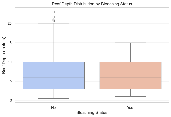
# Plot 2: Distribution of Reef Depth by Bleaching Status
plt.figure(figsize=(8, 5))
sns.boxplot(data=df, x='Bleaching', hue='Bleaching', y='Depth', palette='coolwarm', legend=False)
plt.title('Reef Depth Distribution by Bleaching Status')
plt.xlabel('Bleaching Status')
plt.ylabel('Reef Depth (meters)')
plt.show()<class 'pandas.DataFrame'>
RangeIndex: 9111 entries, 0 to 9110
Data columns (total 12 columns):
# Column Non-Null Count Dtype
--- ------ -------------- -----
0 Bleaching 9111 non-null str
1 Ocean 9111 non-null str
2 Year 9111 non-null int64
3 Depth 9111 non-null float64
4 Storms 9111 non-null str
5 HumanImpact 9111 non-null str
6 Siltation 9111 non-null str
7 Dynamite 9111 non-null str
8 Poison 9111 non-null str
9 Sewage 9111 non-null str
10 Industrial 9111 non-null str
11 Commercial 9111 non-null str
dtypes: float64(1), int64(1), str(10)
memory usage: 1.2 MBNone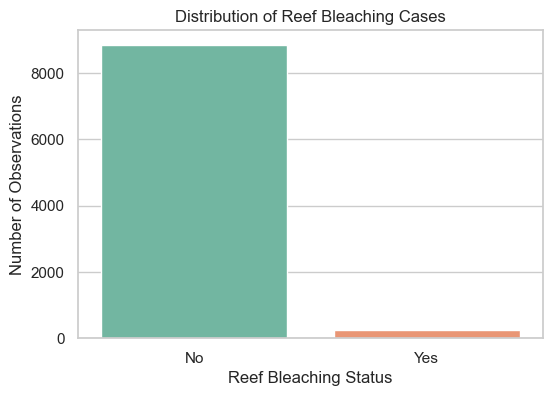
# Convert our compact, balanced sample DataFrame to a string representation for the LLM to understand
df_string = df_sample_compact.to_string()
prompt = f"""
I have the following experimental data:
{df_string}
Please answer the following question about the data:
"""question_1 = "Based on the provided sample, what patterns or commonalities do you notice among the reefs that experienced bleaching (Bleaching = Yes) compared to those that did not (Bleaching = No)?"
full_prompt = prompt + question_1Once you have setup your connection to the API endpoint, you can send your queries with: client.models.generate_content(model='gemini-2.5-flash',contents="My prompt")
response = client.models.generate_content(
    model='gemini-2.5-flash',
    contents=full_prompt
)

print(response.text)
Based on the provided sample data, here are the patterns and commonalities observed between reefs that experienced bleaching (Bleaching = Yes) and those that did not (Bleaching = No):
**Reefs that experienced Bleaching (Bleaching = Yes):**
1. **Year:** These reefs generally appear in earlier years within the sample, specifically 1998, 2001 (three entries), and 2002.
2. **Depth:** A notable commonality is the depth of **10.0 meters**, which accounts for three out of the five bleached reefs. The other two are at 4.0 and 5.0 meters. This suggests a tendency towards deeper reefs in this bleached sample.
3. **Human Impact:** While some had "low" or "moderate" human impact, one instance of bleaching occurred where HumanImpact was recorded as "none."
4. **Sewage:** Three out of five bleached reefs had "none" for Sewage levels, with the others showing "low" or "moderate."
**Reefs that did NOT experience Bleaching (Bleaching = No):**
1. **Year:** These reefs are from more recent years within the sample, ranging from 2006 (two entries) to 2012, 2013, and 2015.
2. **Depth:** These reefs show a wider variation in depth, including several at shallower levels (2.2, 2.5, 3.0 meters), but also deeper ones (10.0, 11.0 meters). There isn't a single dominant depth.
3. **Human Impact:** All reefs in this group had at least some level of human impact, recorded as either "low" or "moderate" (no instances of "none").
4. **Sewage:** These reefs also show a mix of "none," "low," and "moderate" sewage levels.
**Overall Patterns and Commonalities/Differences:**
* **Temporal Trend (Year):** A striking pattern is the **temporal separation**. Bleaching events in this sample are concentrated in earlier years (late 1990s-early 2000s), while the absence of bleaching is observed in later years (mid-2000s-2010s).
* **Depth:** Bleached reefs in this sample lean towards deeper environments (specifically 10m), whereas non-bleached reefs display a broader range of depths, including many shallower ones.
* **Human Impact:** Interestingly, reefs that did not bleach *always* had some level of human impact (low or moderate) in this sample. Conversely, one bleached reef had *no* recorded human impact, suggesting bleaching can occur independently of direct human influence in this dataset.
* **Storms and Ocean:** Both groups show a mix of 'yes' and 'no' for Storms, and a diversity of 'Ocean' types, indicating no clear differentiating pattern for these variables in this sample.
* **Sewage:** Both groups include reefs with "none," "low," and "moderate" sewage, so no strong pattern emerges here.question_2 = "Formulate a hypothesis explaining how human activities (like Sewage or HumanImpact) might interact with natural factors (like Storms or Depth) to influence coral bleaching, using the provided data to support your reasoning."
full_prompt_2 = prompt + question_2
print(f"\nQuestion: {question_2}")
response_2 = client.models.generate_content(
model='gemini-3-flash-preview',
contents=full_prompt_2
)
print("AI Response:")
print(response_2.text)
Question: Formulate a hypothesis explaining how human activities (like Sewage or HumanImpact) might interact with natural factors (like Storms or Depth) to influence coral bleaching, using the provided data to support your reasoning.
AI Response:
Based on the provided experimental data, here is a formulated hypothesis regarding the interaction between human activities and natural factors, supported by specific observations from the dataset:

### **Hypothesis**
**"Natural physical disturbances (Storms) act as a primary catalyst for coral bleaching only when the reef’s resilience has been compromised by human-induced nutrient loading (Sewage). Furthermore, shallow depth may offer a protective effect against these combined stressors, whereas deeper reefs are more susceptible even under lower human impact."**

---

### **Supporting Evidence from the Data**

#### **1. The Interaction of Storms and Sewage**
The data suggests that a storm alone is often insufficient to cause bleaching unless sewage is also present.
*   **Sample 6392:** When a **Storm (Yes)** coincided with **Moderate Sewage**, bleaching occurred (**Yes**).
*   **Sample 8120:** Conversely, when a **Storm (Yes)** occurred but there was **No Sewage**, the coral did not bleach (**No**), even though the general HumanImpact was "moderate."
*   **Sample 5814:** When **Moderate Sewage** was present but there was **No Storm**, bleaching did not occur (**No**).
*   *Reasoning:* This suggests a synergistic effect where sewage weakens the coral’s physiological defenses, making the physical stress of a storm the "tipping point" for a bleaching event.

#### **2. The Role of Depth as a Buffer**
Shallower reefs in this dataset appear to resist bleaching more effectively than deeper reefs when facing similar human pressures.
*   **Sample 8535 (Depth 2.5m):** This reef experienced a **Storm** and **Moderate HumanImpact**, yet it did **not bleach**.
*   **Sample 3477 (Depth 2.2m):** Similarly, this very shallow reef experienced a **Storm** and survived without bleaching.
*   **Sample 2820 & 6685 (Depth 10.0m):** Both of these deeper reefs experienced bleaching (**Yes**) despite having **None** or **Low** human impact/sewage.
*   *Reasoning:* Shallow corals may be more naturally adapted to high-energy environments and light fluctuations, making them more resilient to the turbidity or runoff caused by storms compared to corals at a 10-meter depth.

#### **3. Temporal Trends and Human Impact**
There is a notable shift in the data based on the year, which may reflect changing baseline temperatures or reef acclimation.
*   **Earlier Years (1998–2002):** Almost all samples from this period (424, 6392, 2820, 3120, 6685) resulted in **Bleaching**, regardless of whether the sewage was low or non-existent.
*   **Later Years (2006–2015):** Almost all samples (8120, 3477, 5814, 8535, 5341) showed **No Bleaching**, even in the presence of moderate human impact.
*   *Reasoning:* This might suggest that in later years, only the most severe combinations of factors (like the Storm/Sewage combo in 6392) trigger bleaching, or that the reefs represented in the later data points have higher baseline resilience.

### **Summary Conclusion**
The data indicates that **Sewage** is a critical "sensitizing" factor. While a reef might survive high HumanImpact or a Storm individually, the combination of **Storm-driven physical stress** and **Sewage-driven chemical stress** appears to be a decisive driver for bleaching, particularly as **Depth increases**.
Calling the Gemini API can be done easily with the high-level “genai” package, or you can use the industry-standard baseline OpenAI endpoints to seamlessly swap between model providers.
This simple introductory lesson was just to get you started. With these foundational Python and AI concepts, you can scale up your research workflows significantly! Here are some ideas for how AI may fit into your pipelines:
Models that generate, analyse, and process text or code (e.g., Gemini, ChatGPT, Anthropic’s Claude, Meta’s LLaMA).
Models trained to interpret and analyse visual data.
Models trained on specific types of complex scientific data, like molecular structures, physics simulations, or audio.
Important: The AI landscape is evolving rapidly, and these tools are completely changing how we handle data. Stay curious and experiment with them, but always remain critical. AI models can hallucinate plausible-sounding falsehoods, so human oversight and strict validation of all outputs are non-negotiable.